Potential Energy of Point Charges
The potential energy of two point charges a distance d apart iswhere k=$9\ten9\u{Nm^22/C^2}$ as before. This looks very similar to Coulomb’s Law, but notice the lack of absolute value signs: the potential energy can be positive or negative, and negative PE is considered to be lower than positive PE.
Example

A $+2\u{µC}$ charge starts off a distance 0.4m away from a $+4\u{µC}$ charge, and moves away until it is 1m away. To calculate the change in its potential energy we need the initial and final values: $$\begin{align} \Delta PE &= PE_f-PE_i\\ &= k{q_Aq_B\over d_f} − k{q_Aq_B\over d_i}\\ &= {\color{red}kq_Aq_B}{\color{blue}\left(\frac1d_{\!f} - \frac1d_{\!i}\right)}\\ &= {\color{red}\left(9\ten9\u{Nm^2\over C^2}\right)} {\color{red}(+2\u{\mu C})(+4\u{\mu C})}\\ & \qquad{\color{blue}{\times\left(\frac1{1\u{m}}-\frac1{0.4\u{m}}\right)}}\\ &={\color{red} (+0.072)}{\color{blue}(-1.5)} =−0.108\u{J}\\ \end{align}$$ Because this is negative, the potential energy of the charges decreases, and this makes sense because the two positive charges are moving farther apart, which is exactly what they want to do.
If I replaced the +2µC charge to a –2µC charge, then the change in potential energy would be $\Delta PE = (-0.072)(-1.5) = +0.108\u{J}$. The change is positive, which means a negative charge would not spontaneously start moving away from a positive charge.

This graph shows how the potential energy changes as the particles get farther apart. When both charges are the same sign then $qAqB>0$, and we use the top curve: the energy gets higher and higher the closer the particles are together. Conversely, for opposite charges we use the bottom curve, and the energy gets lower and lower as the particles get closer. In both cases, however, the potential energy approaches zero* as the distance between the charges gets large.
Multiple Charges
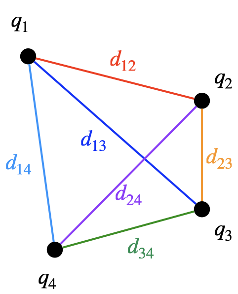
If there are more than two charges, the total potential energy is the sum of the energies from every pair of charges. For instance, if there are four charges, then there are six different pairs to consider: $$\begin{align} PE&={\color{red} k{q_1q_2\over d_{12}}} +{\color{blue} k{q_1q_3\over d_{13}}} +{\color{cyan} k{q_1q_4\over d_{14}}} \\ & +{\color{orange} k{q_2q_3\over d_{23}}} +{\color{purple } k{q_2q_4\over d_{24}}} +{\color{green} k{q_3q_4\over d_{34}}}\\ \end{align}$$